Elliptic curves cheat sheet

Elliptic curves are special mathematical objects commonly defined by a cubic equation of the form \(y2=x3+ax+b \), where a and b are constants. Thanks to their mathematical properties, such as their ability to perform efficient arithmetic operations and the difficulty of solving discrete logarithm problems (DLP) on them, elliptic curves became ubiquitous in modern cryptography. Today, elliptic curves can be found in digital signature schemes (DSA), key exchange mechanisms (KEM), zero-knowledge proofs (ZKP), multi-party computation (MPC), and more.

This cheat sheet provides a brief overview of the parameters that define an elliptic curve and offers a somewhat opinionated classification of existing elliptic curves.

Anatomy of elliptic curves

The most defining characteristic of elliptic curves is their endomorphism ring, which is also the most abstract one. Namely, it's a set of mathematical operations that can be performed on the curve. These operations include point addition and scalar field multiplication, and they give information about the curve's properties.

Order \(n\) is the maximum number of points on the curve and is sometimes called cardinality.

Base field \(F_q\) of an elliptic curve is the field over which the curve is defined. The base field size \(q\) thereby defines the number of elements of the finite field \(F_q\).

Scalar field \(F_r\) is the field of scalars used in the operations performed on the curve, such as point addition, scalar multiplication, and pairing. The scalar field size \(r\) is also the size of the largest subgroup of prime order. Interestingly, the Elliptic Curve DLP (ECDLP) of an elliptic curve is only as hard as that curve's largest prime order subgroup, not its order. However, when the curve's order is prime, its largest prime subgroup is the group itself, so \(r=n\).

The following are three parameters that give an impression of the curve's security and performance:

Relative parameter

\[ρ=logq/logr\]

Relative parameter measures the base field size relative to the size of the prime-order subgroup on the curve. Small ρ is desirable to speed up arithmetic on the elliptic curve.

Cofactor

\[h=n/r\]

Cofactor measures the curve's order relative to its largest prime subgroup. The cofactor of prime-order curves is always equal to 1. There's a trade-off where curves with cofactor tend to have faster and simpler formulas than those of prime-order curves, but are also more likely to be vulnerable to certain attacks, such as malleability.

Trace of Frobenius

\[q+1−r\]

Trace of Frobenius describes the size of a reduced curve. It's used to better estimate the security of the elliptic curve and is useful when finding new curves with desirable properties.

The embedding degree is the smallest integer \(k\) that lets you transform an instance of the ECDLP over an elliptic \(E(F_q)\) into an instance of the DLP over the field \(F_qk\). It's particularly important because the best known ECDLP attack \(O(√n)\) is Pollard's rho, while the best DLP attack is Index Calculus, being sub-exponential in the field size. This kind of reduction is possible with pairing-friendly curves, so their \(qk\) must be significantly larger than order n. When \(k>1\) we say that curve is defined over extension field of size \(qk\).

Security bits \(s\) measure the difficulty of solving the DLP on a curve. For plain curves, \(s\) is roughly \(log2r\). For pairing-friendly curves, \(r\) must be selected such that \(log2r≥2s\) because of Pollard's rho algorithm, but due to the ambiguity of Index Calculus attack complexity, estimating s isn't as trivial:

$$
2^{v} \cdot e\left(
\sqrt[3]{ \tfrac{c}{9} \cdot \ln(kq) \cdot \bigl[\ln(\ln(kq))\bigr]^{2} }
\right)
$$

...where the constants \(c=32\) and \(v=−7\) (source).

Primitive point \(G\) is a generator of the group \(F_q\): all elements of the group can be expressed as \(G+G+...+G\) (up to \(q\) times). If a curve's order is prime, then all its points (except the point at infinity) are primitive.

Taxonomy of elliptic curve groups

There are many ways to classify elliptic curves: by their algebraic structure, geometric shape, cryptographic properties, security levels, etc. Let's start by looking at the properties of their endomorphism rings.

By the properties of their endomorphism rings

Ordinary elliptic curves have the endomorphism ring that is isomorphic (equivalent) to the ring of integers of a number field, i.e. all points are in the set of real integers.

Supersingular curves are elliptic curves whose order is not divisible by the characteristic of the field (the smallest positive integer m such that for all elements a in the field, \(a+a+...+a (n times) = 0\).

Complex multiplication (CM) elliptic curves are curves whose points are created by multiplying their generator point by the complex multiplication constant. They naturally have a large number of points and can be used to generate large prime-order subgroups.

Pairing curves are defined by a pair of elliptic curves \(G_1\), \(G_2\) and a bilinear map between their respective groups of points that maps their points \(G_1×G_2→G_T\). Curves with a small embedding degree \(k<40\) and a large prime-order subgroup \(ρ≤2\) are called pairing-friendly curves.

By their definition form

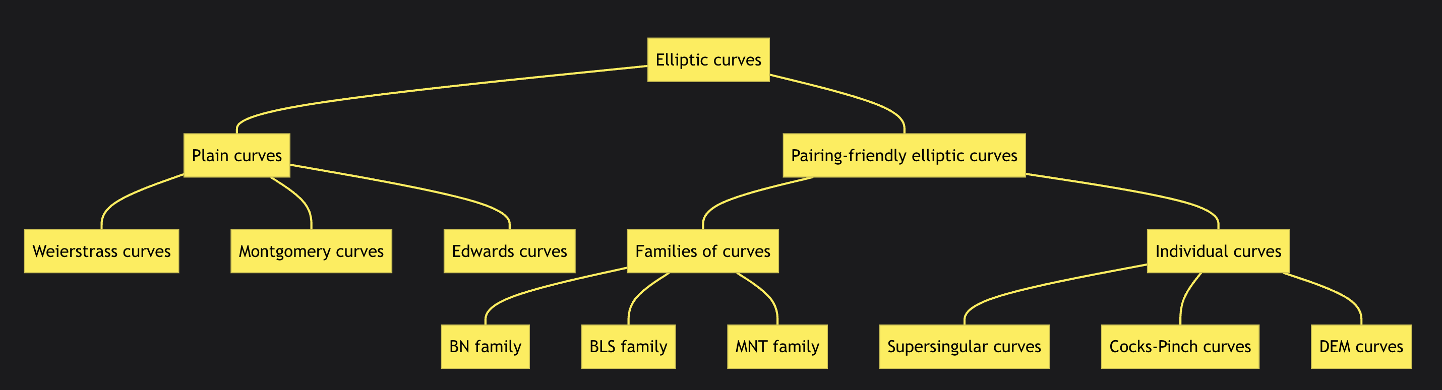
Weierstrass curves are defined as \( y^2 = x^3 + Ax^2 + B \). This is arguably the most common form for elliptic curves. Weierstrass curves initially lack full addition and were slower, but the gap has closed over time. Examples are the BLS family (BLS12-381, BLS12-377).

Montgomery curves are defined as \(By^2 = x^3 + Ax^2 + x\). These curves are very efficient for elliptic curve multiplication (ECM). They are explicitly designed to work well with the Montgomery ladder. Using this algorithm, it's possible to multiply any two points without failure cases. There are faster methods to multiply a variable point by a fixed one. Still, the Montgomery ladder is very effective for multiplying two arbitrary points. A notable example is Curve25519.

Edwards curves are defined as \(Ax^2 + y^2 = 1 + Dx^2 * y^2\). Such curves gained huge popularity because they were the first to implement the full addition law, i.e. allowed to efficiently add any two points without failure cases. Complete addition formulas can simplify the task of an ECC implementer and, at the same time, can significantly reduce the potential vulnerabilities of a cryptosystem. An example of an Edwards curve is Ed25519.

Twisted Edwards curves are a type of Edwards curve. They include a special affine transformation that twists the curve. This makes some operations, like the Elligator map and hash to curve, more efficient. Curves of this form are birationally equivalent to Montgomery curves. People often specify the Montgomery curve first and then transform it into Twisted Edwards form. Notable examples are Ed-on-BLS12-381, aka JubJub, and Ed-on-BN254, aka Baby-Jubjub.

Elliptic curve fields: base field and scalar field explained

Elliptic curves are defined over two fields of finite order: the base field represents points on a curve, while the scalar field allows performing scalar multiplication on those points.

Characteristics such as relative parameter \(ρ\), cofactor, and trace can say a lot about the curve's security and performance. Estimating security bits of a given curve is generally trivial for plain curves, but can be quite troublesome for pairing-friendly curves.

Elliptic curves can be classified by their endomorphism rings or by their definition form. There are ordinary, supersingular, CM, and pairing-friendly curves. Each type has a different endomorphism ring structure. When it comes to defining elliptic curve equations the most popular ways are Weierstrass, Montgomery, Edwards, Twisted Edwards forms.